Relativistic Knot Theory: Topology in the Minkowski Metric Sheet

Started: 2025-11-30

Relativistic knot theory sounds like a topic for a sci-fi novel—knots tied in the fabric of spacetime, constrained by the speed of light. While the field exists in mathematical physics (studying knotted worldlines, cosmic strings, and vortex tubes), I recently stumbled into it from a completely different direction: Distance Matrix Analysis.

By swapping the standard Euclidean metric for the Minkowski metric in a pairwise distance analysis, we uncover a fascinating topological structure. It turns out that the “over/under” crossings of a knot are naturally encoded in the causal structure of its points.

The Shift: From Object to Relation

Classical knot theory looks at embeddings of a circle $S^1$ into $\mathbb{R}^3$. We usually visualize this via 2D projections, counting crossings and checking for isotopies (deformations).

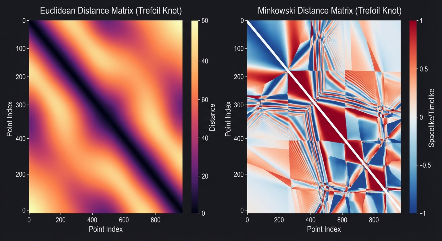
However, we can also look at a knot purely through its Distance Matrix—the set of all pairwise distances between points on the curve. $ D_{ij} = |x_i - x_j| $ Figure 1: A comparison of the pairwise distance matrix for a Trefoil knot. Left: The standard Euclidean metric creates a smooth landscape. Right: The Minkowski metric reveals a complex causal structure with sharp boundaries separating timelike and spacelike regions.

In Euclidean space, this matrix is just a smooth, hilly landscape. It tells us about geometry, but the topology is subtle. However, if we embed the knot in a 2+1 dimensional spacetime and apply the Minkowski Metric: $ s^2 = -c^2(t_i - t_j)^2 + (x_i - x_j)^2 + (y_i - y_j)^2 $

The landscape changes dramatically. The distance is no longer just a magnitude; it has a sign.

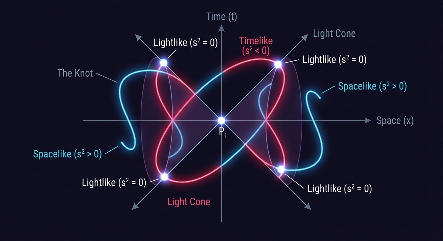
$s^2 < 0$: Timelike (Causally connected)
$s^2 > 0$: Spacelike (Causally disconnected)
$s^2 = 0$: Lightlike (On the light cone)

Figure 2: The 'Z-buffer' of topology. By determining if a distant point lies inside, outside, or on the light cone of the observer, the Minkowski metric encodes the relative ordering of the knot's strands.

This sign structure acts as a “Z-buffer” for topology. It encodes the ordering of points in a way that captures the notion of “over” and “under” without needing a projection plane. If $s^2(A, B) < 0$ and $t_A > t_B$, then $A$ is in the absolute future of $B$. This causal ordering fixes the relative depth of the strands, turning topological ambiguity into causal certainty.

The Hierarchy of Constraints

In exploring this via the interactive lab, a profound distinction emerged between the physics of the curve and the topology of the sheet.

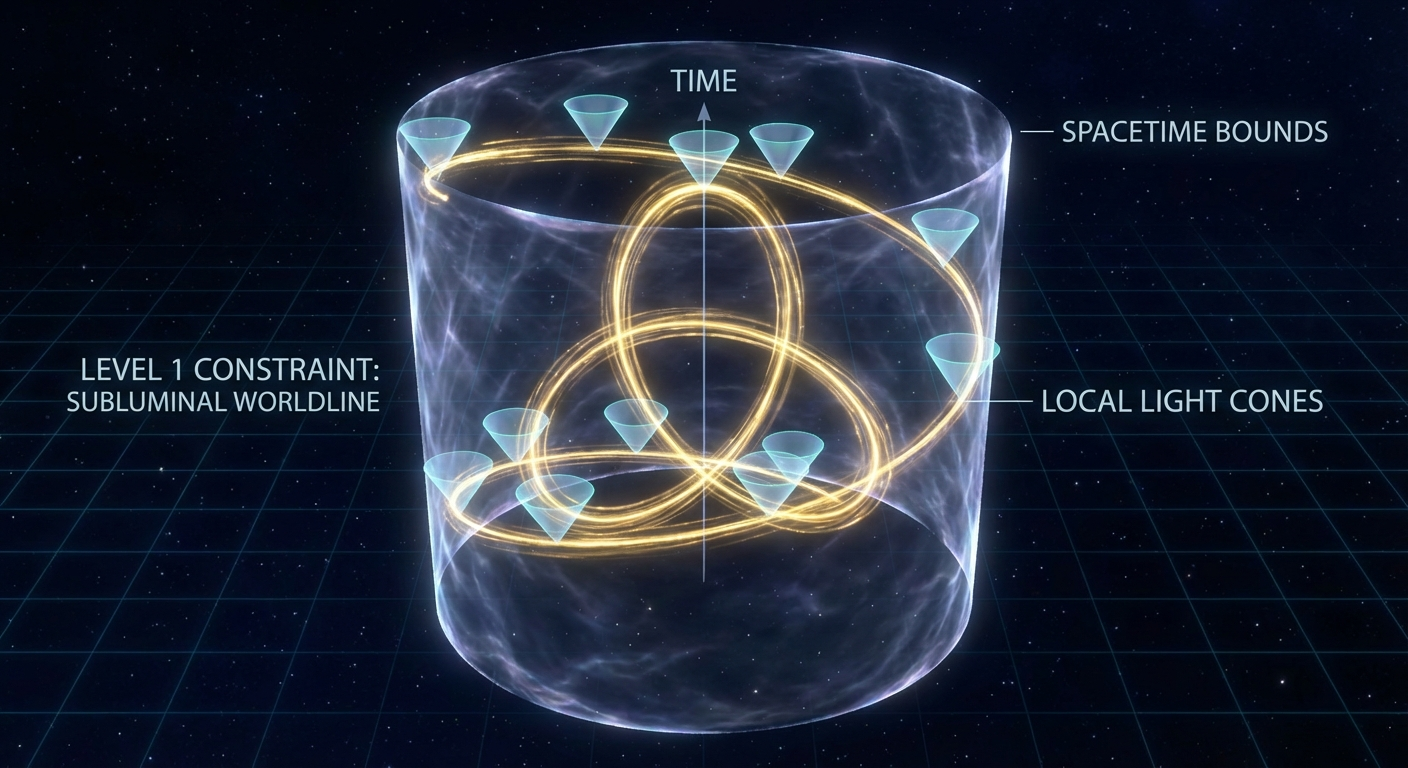
Level 1: The Curve (The Worldline)

If we view a knot as a particle’s path through spacetime (a worldline), we might ask: “Is this knot possible? Does it violate the speed of light?”

Critique of “Worldlines”: The terminology “worldline” is slightly misleading here. A worldline usually implies a particle’s history. A better physical analogue might be a vortex ring in a relativistic fluid or a cosmic string loop at a specific instant, extended into spacetime. The analysis treats the knot as a static 4D object rather than a dynamic evolution.

It turns out that for a closed knot to exist in Minkowski space, the answer is “Yes, but it must be superluminal.” Because a knot is a closed loop, the particle must eventually return to its starting time coordinate. This implies that $\oint dt = 0$, which is impossible for a strictly subluminal particle (which always moves forward in time).

Therefore, these “Minkowski Knots” trace worldlines that are largely, if not wholly, spacelike (non-causal). This creates a sort of Grandfather Paradox of Knots: To trace a knot in spacetime and return to where you started, you must eventually travel faster than light (or back in time).

The “Timelike Islands” we see in the distance matrix aren’t just abstract features; they represent the specific regions where you are effectively time-traveling to cross “under” the rope. The structure we are analyzing is essentially the causal footprint of a tachyon or a static string, not a standard particle. Figure 3: A knotted worldline in spacetime. Unlike a standard particle, a closed knotted worldline must exit the light cone to return to its past, making it an inherently superluminal or acausal structure.

Level 2: The Metric Sheet

However, if we look at the Metric Sheet—the surface defined by the pairwise Minkowski distances of all points $(s_1, s_2)$—the story changes.

The topology of the knot is encoded in the level sets and sign changes of this sheet. We define the sheet function $F$ on the torus of parameters $[0, L] \times [0, L]$: $ F(s_1, s_2) = \text{MinkowskiMetric}(\gamma(s_1), \gamma(s_2)) $

Here is the core insight: While the curve can avoid the light cone locally (tangent vectors remain inside the cone), the metric sheet cannot avoid it globally (secant vectors must cross the cone).

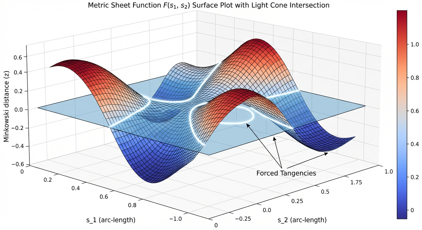
Consider the map $\Phi: T^2 \to \mathbb{R}^{2,1}$ defined by the difference vectors $v(s_1, s_2) = \gamma(s_1) - \gamma(s_2)$. The metric sheet is essentially the pullback of the light cone structure through this map. For non-trivial knots, the image of the torus $T^2$ wraps around the origin in such a way that it must intersect the light cone surface non-trivially. Figure 4: The Metric Sheet. The topology of the knot is captured not by the curve itself, but by how the pairwise distance surface intersects the zero-plane (the light cone). Non-trivial knots force specific intersection patterns that cannot be smoothed away.

For a non-trivial knot (like a Trefoil), the metric sheet is forced to have tangencies or specific intersection patterns with the “light cone rays” (where $s^2=0$) in the target space. You cannot homotope these tangencies away without untying the knot.

This provides a rigorous definition of knot complexity based on negative space: A knot is non-trivial if its pairwise causal structure cannot avoid intersecting the light cone in specific, structured ways.

Proof Sketch: The Timelike Island

Why is this structure rigid? We can prove it by looking at the nature of a “crossing.”

The Crossing is Timelike: In a standard spatial projection, a crossing occurs where two distinct points on the curve, $u$ and $v$, share the same spatial coordinates $\vec{x}$ but exist at different times $t$. $\Delta \vec{x} = 0, \quad \Delta t \neq 0 \implies s^2 = -c^2\Delta t^2 < 0$ This creates a “valley” of negative (timelike) distance in the matrix.
The Bulk is Spacelike: For a sufficiently large knot or a sufficiently fast (superluminal) traversal, the majority of point pairs are separated by space, not time. $|\Delta \vec{x}| > c|\Delta t| \implies s^2 > 0$ This forms the “plateau” of positive (spacelike) distance.
The Inevitable Boundary: By the Intermediate Value Theorem, any continuous path on the parameter torus connecting a crossing point $(u, v)$ to a generic bulk point must pass through $s^2 = 0$. Therefore, every topological crossing in the knot manifests as a Timelike Island surrounded by a Lightlike Shoreline ($s^2=0$) within the metric sheet. You cannot remove the crossing without merging the island into the mainland (unknotting) or collapsing the time dimension.
Topological Stability: These islands are not merely artifacts of a specific parameterization. They correspond to the critical points of the distance function. In Morse theory terms, the creation or annihilation of these timelike islands corresponds to Reidemeister moves. Specifically, a Reidemeister II move (creating two crossings) appears as the birth of a pair of timelike islands (one positive, one negative in terms of oriented crossing sign) from the spacelike sea.

The “Minkowski Number”

Standard knot invariants include Jones Polynomials or Crossing Numbers. This framework suggests a new physical invariant: the Minkowski Number. Defined as the minimum volume of the “Timelike Islands” required to represent a specific knot type (normalized by arc length), it quantifies “how much causality must be violated” to tie a specific knot. A trivial knot (unknot) has a Minkowski Number of 0, as it can be deformed to lie entirely in a spacelike slice.

Visualizing the Theory

I built a WebGL simulation to explore this directly.

Launch the Interactive Lab

Figure 5: The Interactive Topology Lab. Rotating the 'Time' axis changes the metric signature, causing the causal horizon to sweep across the knot and altering the topology of the distance matrix in real-time.

In the lab, you can:

Generate Knots: Trefoils, Figure-8s, and random splines.
Rotate Time: The visualization allows you to rotate the axis designated as “Time.” This isn’t just rotating the object; it changes the metric signature of the space.
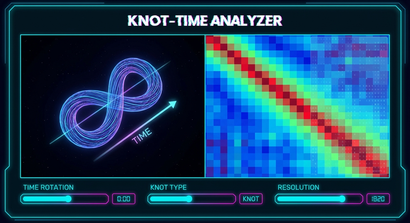
View the Matrix: Watch the distance matrix transform from a Euclidean hill to a Minkowski landscape.

As you rotate the time axis, you can see the “causal horizon” sweep across the knot. The ridges and valleys in the distance matrix shift, revealing the invariant structure of the knot not as a shape in space, but as a pattern of causal relationships.

Implications

This approach reframes relativistic knot theory. Instead of asking “How does this knot look to an observer?”, we ask “ What is the topology of the causal relationships between all points on this knot?”

It suggests a two-tier reality for relativistic systems:

Parametrization (Physics): Flexible. We can move how we like, provided we stay subluminal.
Relational Structure (Topology): Rigid. The web of causal connections forms a sheet that is pinned to the light cone structure of the universe.

This is a perfect example of incentive-shaped topology: the “incentive” is the speed of light, and the “topology” is the set of configurations that cannot escape that constraint.

Feature	Consideration	Risk	Opportunity
Metric Rotation	Rotating the “Time” axis is a linear transformation of the input coordinates.	High CPU-GPU bus latency if coordinates are re-uploaded every frame.	Perform the rotation matrix multiplication directly in the Vertex/Fragment shader.
Timelike Islands	These are the “features” of the knot.	Aliasing: Small islands might disappear at low resolutions.	Use Signed Distance Fields (SDFs) to represent the knot, allowing for sub-pixel island detection.
Minkowski Number	Needs normalization by arc length.	Numerical instability if the knot has high-frequency “wiggles.”	Use this as a Machine Learning feature for rapid knot classification (faster than Jones Polynomials).

The Causal Knot: Decoding Topology via Minkowski Distance Matrices

This tutorial explores the intersection of knot theory and special relativity. You will learn how to transform a standard 3D knot into a 2+1 dimensional spacetime worldline and use the Minkowski metric to generate “Causal Distance Matrices.” By the end of this lab, you will understand how the “over/under” crossings of a knot are naturally encoded in the causal structure of spacetime, acting as a topological “Z-buffer.”

⏱️ Estimated Time: 45 minutes

🎯 Skill Level: Intermediate

💻 Platform: Web Browser / WebGL Lab

What You’ll Learn

✓ Contrast Euclidean and Minkowski distance matrices in the context of curve analysis. ✓ Identify timelike, spacelike, and lightlike regions within a pairwise distance plot. ✓ Explain how causal ordering ($s^2 < 0$) resolves topological ambiguity in knot projections. ✓ Manipulate spacetime parameters (like the constant $c$) to observe how they alter the topological “visibility” of a knot.

Prerequisites

Required

Modern Web Browser (software): Chrome, Firefox, or Edge with WebGL 2.0 support.
- Download:
3D Coordinates (knowledge): Basic understanding of 3D coordinates (x, y, z).
- Download:
Distance Matrix Concepts (knowledge): Familiarity with the concept of a “distance matrix” (pairwise distances between points).
- Download:
Special Relativity Basics (knowledge): Introductory knowledge of Special Relativity (specifically the concept of a light cone).
- Download:

Optional

GPU Hardware (hardware): A device with a dedicated or integrated GPU is recommended for smooth WebGL rendering.
- Download:

Tutorial Steps

Step 1: Initializing the Knot Lab and 3D Visualization

Before analyzing a knot through the lens of relativistic causal structures, you must first establish its baseline geometry in standard 3D Euclidean space. This step initializes the simulation environment and loads the Trefoil Knot—the simplest non-trivial knot—to serve as our primary topological subject. Understanding its spatial ‘over/under’ crossings in a static 3D environment is essential for later interpreting ho## Generation Complete

Statistics:

Total Steps: 6
Prerequisites: 5
Word Count: 4040
Code Blocks: 2
Total Time: 281.533s

Completed: 2026-03-03 12:45:49 onfiguration panel, select the ‘Trefoil Knot (3_1)’ preset and click Apply/Generate. Finally, use the viewport controls (rotate, zoom, pan) to inspect the knot and identify the three distinct crossing points where the curve passes over or under itself.

Parametric equations for the Trefoil Knot (p=2, q=3)

x = sin(t) + 2*sin(2*t)
y = cos(t) - 2*cos(2*t)
z = -sin(3*t)

📸 The Geometry Configuration panel with ‘Trefoil Knot’ selected and the Apply button highlighted.

📸 A high-contrast 3D view of the Trefoil knot, showing a clear ‘over’ crossing where the z-depth difference is visible.

Expected Outcome: You should see a continuous, self-intertwined loop rendered in the 3D viewport. The knot should appear as a smooth, tubular structure with no breaks. You should clearly identify three locations where the ‘strand’ crosses another, creating the characteristic clover-like shape of the Trefoil (3_1 knot).

Verify Success:

Rotate the model 360 degrees and verify that there are exactly three points where one segment of the knot clearly passes over another.
Follow the path of the knot with your eyes to ensure it is a single closed loop with no loose ends.
Hover the cursor over a crossing to verify that the two segments have similar X and Y values but distinct Z values.

⚠️ Common Issues:

Blank Viewport: If the 3D view is black, ensure WebGL2 and hardware acceleration are enabled in browser settings.
Stuttering Performance: If rotation is laggy, reduce ‘Segment Resolution’ or ‘Point Count (N)’ to 100 in the Settings panel.
Knot Looks Like a Circle: Ensure ‘Trefoil Knot’ is selected in the preset menu rather than ‘Unknot’.
Z-Fighting at Crossings: If segments flicker at crossings, increase the Z-Scale slider to create more vertical separation.

Step 2: Generating the Euclidean Distance Matrix

Before we introduce the complexities of Minkowski spacetime, we must establish a geometric baseline. In this step, you will generate a Euclidean Distance Matrix (EDM). This matrix represents the ‘classical’ way of looking at a knot: it treats the knot as a static object in 3D space and calculates the straight-line distance between every possible pair of points along the curve. This helps us understand the knot’s spatial density and proximity without the influence of time or light-cones.

To perform this step:

Toggle the Matrix View to Euclidean Mode in the ‘Analysis Controls’ overlay. This calculates distances using the standard Pythagorean metric.
Observe the Heatmap Generation in the secondary 2D viewport, where X and Y axes represent the parameter t from 0 to 2π.
Identify the Main Diagonal (top-left to bottom-right), which represents the distance of a point to itself (zero).
Analyze the Smooth Gradients radiating from the diagonal, representing the flow of the curve.

📸 A split-view showing the 3D Trefoil knot on the left and a colorful, perfectly symmetric 2D heatmap on the right. The heatmap shows a dark diagonal line with soft, undulating patterns of color.

Expected Outcome: You will see a symmetric heatmap. Because the distance from Point A to Point B is the same as Point B to Point A in Euclidean space, the top-right triangle of the matrix is a mirror image of the bottom-left. The heatmap will appear ‘soft’ or ‘blurry’, showing where strands get close but lacking clear topological crossing data (over/under).

Verify Success:

Symmetry Check: Hover your cursor over the matrix at coordinates (i, j) and then (j, i). The ‘Distance Value’ readout in the status bar should be identical for both.
Continuity Check: Ensure there are no jagged ‘staircase’ artifacts in the gradients. If the matrix looks pixelated, increase the Sample Resolution slider in the settings to at least 512.
Zero-Diagonal: Confirm that the diagonal is a solid line of zero distance.

⚠️ Common Issues:

Matrix is Blank/Black: This often occurs if the WebGL fragment shader fails to compile. Check the ‘Developer Console’ (F12) for ‘Shader Link Errors.’ Refreshing the page usually resolves this.
Low Contrast: If the heatmap looks washed out, adjust the Distance Scaling or Gamma slider in the Matrix View settings.
Performance Lag: If the 2D view is stuttering, you may be calculating too many points. Reduce the Matrix Resolution to 256 x 256 for smoother real-time interaction.

Step 3: Embedding the Knot in 2+1 Spacetime

The core of Relativistic Knot Theory lies in the transition from static 3D geometry to a dynamic 2+1 Spacetime framework. In this step, you will redefine the Z-axis of your visualization. Instead of representing a third spatial dimension, the Z-axis will now represent Time (t). This transformation converts the knot from a simple loop into a Worldline—the complete history of a point particle moving and interacting in a 2D plane over a specific duration.

Actions:

Locate the Spacetime Toggle: Navigate to the Visualization Settings panel on the right side of the WebGL interface. Look for the section labeled ‘Coordinate Mapping’.
Enable ‘Spacetime Embedding’: Click the toggle switch labeled Spacetime Embedding (Z → t). Note: You may notice the knot instantly ‘stretch’ along the vertical axis.
Adjust the Temporal Scale (Optional): If the knot appears too compressed or too elongated to analyze, use the Time Scale Slider (often labeled c or Δt) to adjust the vertical stretching.
Observe the Worldline Transformation: Rotate the camera using your mouse (Left-Click + Drag) to view the knot from the side. Observe how the continuous loop now flows from the bottom (the ‘Past’) to the top (the ‘Future’).
Identify Causal Directionality: Trace the path of the strand starting from the lowest point on the Z-axis. As you follow the strand ‘upward,’ you are tracing the chronological history of the particle.

📸 A side-by-side comparison of the Trefoil knot. On the left, the standard 3D Euclidean knot. On the right, the elongated ‘Spacetime’ version where the Z-axis is significantly stretched and labeled ‘Time’.

📸 Close-up of a crossing in Spacetime mode, showing one strand clearly ‘above’ (later in time) than the strand it crosses.

Expected Outcome: The knot will no longer appear as a compact, balanced object. Instead, it will look like an elongated helix or a ‘stretched spring’ that has been tangled. The vertical axis (Z) now represents the progression of time. You should be able to visually distinguish between ‘earlier’ events (lower on the screen) and ‘later’ events (higher on the screen). The concept of a Worldline becomes apparent: the knot is now a record of a 2D point’s journey through time.

Verify Success:

Verticality Check: Ensure that the Z-axis is oriented vertically. In this mode, ‘Up’ must strictly represent the future.
Coordinate Readout: Hover your mouse over a point on the knot. The tooltip should now display coordinates as (x, y, t) instead of (x, y, z).
Loop Continuity: Verify that the strand still forms a closed loop. In relativistic terms, this represents a ‘Closed Timelike Curve’ (CTC) or a periodic history.

⚠️ Common Issues:

Knot Disappears: If the knot vanishes when you toggle the setting, your ‘Time Scale’ might be set to zero or an extreme value. Reset the slider to the default (1.0).
Perspective Confusion: If the knot looks like a flat 2D circle, your camera is likely positioned directly above the Z-axis (Top-Down view). Rotate the camera to a side view to see the temporal progression.
Performance Lag: On some mobile browsers, the coordinate transformation might cause a brief stutter in the WebGL frame rate. Wait a moment for the shaders to recompile the new vertex positions.

Step 4: Calculating the Minkowski Metric

In this step, you will replace the Euclidean metric with the Minkowski metric to understand the causal structure of the knot. This transforms the distance matrix into a map of causality, revealing which parts of the knot are timelike, spacelike, or lightlike in relation to one another. You will adjust the C-Factor to set the light cone slope and observe how the matrix displays sharp boundaries representing the speed of light limit.

Example logic for the Minkowski Matrix Shader

Run in: ``

function calculateMinkowski(pointA, pointB, c) {
    float dt = pointA.t - pointB.t;
    float dx = pointA.x - pointB.x;
    float dy = pointA.y - pointB.y;
    
    // The Minkowski Metric: s^2 = -c^2 * dt^2 + dx^2 + dy^2
    float s2 = -(c * c) * (dt * dt) + (dx * dx) + (dy * dy);
    
    return s2;
}

📸 Matrix_Comparison_View: A side-by-side comparison. On the left, the blurry Euclidean matrix from Step 2. On the right, the high-contrast Minkowski matrix showing distinct triangular and diamond-shaped causal regions.

📸 Light_Cone_Boundary_Detail: A close-up of the matrix diagonal showing the sharp ‘X’ shapes where the worldline enters and exits the light cone of a specific point.

Expected Outcome: The matrix will no longer look like a continuous heatmap. Instead, it will resemble a complex, geometric pattern of “causal diamonds.” You should see a clear, dark band running down the main diagonal (representing the knot’s local causal connection to its own immediate past and future) and isolated “islands” where the knot loops back through space and enters the light cone of a distant segment.

Verify Success:

Check the Diagonal: The main diagonal (where i=j) should be exactly 0.
Verify Symmetry: The matrix should still be symmetric across the diagonal (s^2_ij = s^2_ji).
Test C-Factor Sensitivity: Move the C-Factor slider to the right (increase c). You should observe the ‘Timelike’ (dark) regions expanding, as a faster speed of light allows more points to become causally connected.

⚠️ Common Issues:

Matrix is Solid Black/White: Your C-Factor may be set too high or too low. If c is near zero, everything is spacelike. If c is infinite, the metric reverts to a quasi-Euclidean state. Reset c to 1.0.

Inverted Colors: If the diagonal is bright instead of dark, your shader is likely plotting

s^2

or has the sign convention flipped (s^2 = c^2t^2 - x^2 - y^2). Ensure the Sign Convention toggle is set to (-, +, +).

Aliasing/Jitter: If the boundaries look ‘pixelated,’ increase the Matrix Resolution slider to 512x512 or higher to better resolve the light-cone intersections.

Step 5: Decoding the “Z-Buffer” of Topology

In standard 3D computer graphics, a “Z-buffer” determines which pixels are in front of others based on their distance from the camera. In Relativistic Knot Theory, we replace this simple depth check with the Minkowski Metric. This step teaches you how to use the sign of the Minkowski interval ($s^2$) to determine the causal “over-under” relationship of the knot’s strands. By the end of this step, you will understand that a “crossing” in a knot is not just a visual overlap, but a specific causal state where one segment of the worldline enters the light cone of another.

Actions:

Locate and Hover Over a “Causal Island”: In the Minkowski Matrix generated in Step 4, look for regions of high contrast away from the main diagonal. Move your cursor over one of these off-diagonal “islands” in the Matrix Viewport and observe the Coordinate Readout (i and j) and the glowing markers in the 3D WebGL Viewport.
Analyze the Causal State: While hovering, look at the Causal Analysis Panel. Identify the calculated value for Δs² (Δx² + Δy² - c²Δt²) and check the Causal Classification (Timelike, Spacelike, or Lightlike).
Correlate Timelike Regions with Physical Overlaps: Rotate your 3D Viewport to look down the Z-axis (Time axis). Find a visual “crossing”, locate the corresponding coordinates in the Minkowski Matrix, and observe that Timelike regions (s² < 0) correspond to these overlaps. Note the Temporal Direction to define the “under” strand.

📸 A split-view showing the Minkowski Matrix on the left and the 3D Knot on the right. A cursor is hovering over a dark blue ‘island’ in the matrix, and two corresponding points are highlighted on the knot where a crossing occurs.

📸 Close-up of the ‘Causal Analysis Panel’ showing a negative $s^2$ value and the label ‘TIMELIKE - CAUSALLY LINKED’.

Expected Outcome: You should see a direct mathematical correlation between the colors in your matrix and the physical geometry of the knot. You will realize that the “Timelike” regions are the “logical glue” of the knot’s topology; they indicate where the worldline is “aware” of its own past or future. The Minkowski metric acts as a logical check: if $s^2$ is negative, the “Z-buffer” is active, and a topological crossing is formally defined.

Verify Success:

Confirm that when you hover over a clear visual crossing in the 3D view, the $s^2$ value in the UI turns negative.
Hover over the main diagonal of the matrix. The value should be $s^2 = 0$ (or very close to it), as a point has zero distance from itself in spacetime.
Press [L] on your keyboard to toggle the “Visual Light Cone” overlay. Ensure the “Future” point of a crossing lies within the translucent cone emanating from the “Past” point.

⚠️ Common Issues:

“Everything looks Spacelike”: If your matrix is entirely $s^2 > 0$, your “Time Scale” constant ($c$) might be set too high. Go to the Constants Slider and decrease the value of $c$. This “shrinks” the light cones, making it harder for points to be causally connected.
Matrix Resolution is Blurry: If the “islands” are hard to pick out, increase the Matrix Sampling Rate in the settings to 512x512 or higher. Note: This may impact WebGL performance on integrated GPUs.
Inverted Overlays: If the “under” strand is showing as “Future,” ensure your Z-axis is not inverted in the Viewport Settings. By convention, +Z should represent increasing time.

Step 6: Stress-Testing the Speed of Light ($c$)

In this step, you will manipulate the ‘Speed of Light’ parameter to observe how the topology of a relativistic knot is relative to the speed of information transfer. The constant $c$ acts as a scaling factor for the temporal dimension in the Minkowski interval formula: $s^2 = \Delta x^2 + \Delta y^2 - (c \Delta t)^2$.

First, locate the ‘c (Speed of Light)’ slider in the Parameter Settings panel. By decreasing $c$, you will observe the ‘causal disconnection’ of the knot as the $-(c\Delta t)^2$ term vanishes and the metric reverts to a purely spatial Euclidean distance, causing Timelike regions in the matrix to shrink. By increasing $c$ to its maximum, you reach the Euclidean limit where information travels instantaneously, causing the matrix to be dominated by Timelike connections and the Light Cones to encompass nearly the entire geometry.

📸 A matrix view where the dark timelike bands have narrowed significantly, leaving mostly bright “spacelike” regions.

📸 A matrix view that is almost entirely dark/uniform, indicating that nearly all points are causally connected.

Expected Outcome: By the end of this experimentation, you should see visual proof that topology is a function of $c$. At low $c$, the knot is ‘fragmented’ into causally isolated segments. At high $c$, the knot behaves like a classical 3D string. At the ‘Goldilocks’ $c$ (the default), the matrix reveals the unique ‘Z-buffer’ of relativistic crossings that define Relativistic Knot Theory.

Verify Success:

Check the Interval: Hover your mouse over a previously ‘Timelike’ pixel in the matrix while $c$ is at minimum. The tooltip should now show a positive $s^2$ value (Spacelike).
Visual Sync: Ensure that as you move the slider, the 3D ‘Light Cone’ overlays in the WebGL viewport expand and contract in real-time.
Matrix Contrast: Verify that the ‘Causal Horizon’ (the boundary where $s^2 = 0$) shifts position relative to the knot’s loops.

⚠️ Common Issues:

Lag/Stutter: If the matrix does not update smoothly, lower the ‘Matrix Resolution’ setting in the ‘Performance’ tab.
Inverted Colors: If the matrix turns bright when you increase $c$, check the metric signature and toggle the ‘Invert Metric’ checkbox if necessary.
Vanishing Knot: Avoid setting $c$ to exactly 0 to prevent ‘Division by Zero’ or ‘NaN’ errors in the shader; keep it slightly above 0.01.

Troubleshooting

1. WebGL Context Loss or “Black Screen” on Initialization

Symptoms:

The 3D viewport remains black
The browser console displays WebGL: CONTEXT_LOST_WEBGL

Possible Causes:

Hardware acceleration is disabled in the browser.
The GPU is overwhelmed by the initial distance matrix calculation.
Incompatible browser version for high-precision floating-point textures.

Solutions:

Enable Hardware Acceleration: Go to your browser settings (e.g., chrome://settings/system) and ensure “Use graphics acceleration when available” is toggled ON.
Check WebGL2 Support: Open your console and type const canvas = document.createElement(‘canvas’); console.log(canvas.getContext(‘webgl2’));. If it returns null, update your browser or GPU drivers.
Reduce Initial Resolution: If the lab fails on load, append ?res=low to the URL (if supported) or manually decrease the KNOT_SAMPLES constant in the initialization script to 500 before running.

2. “Imaginary Distance” or NaN Errors in Minkowski Calculations

Symptoms:

The visualization disappears or turns bright magenta when adjusting the $c$ (speed of light) slider.
Console shows Error: Square root of negative value in Minkowski metric.

Possible Causes:

In Relativistic Knot Theory, the interval $s^2 = c^2\Delta t^2 - (\Delta x^2 + \Delta y^2)$ can be negative (spacelike).
Attempting to take the square root of a spacelike interval without handling absolute values or complex components.

Solutions:

Check the Metric Sign Convention: Ensure your code uses the “mostly minus” metric (+ - -) or “mostly plus” (- + +) consistently.
Implement Absolute Mapping: When visualizing distances, use sqrt(abs(s_squared)) to represent the magnitude, and use a color fragment shader to distinguish between Timelike (blue) and Spacelike (red) intervals.
Clamp $c$ Values: Ensure the $c$ slider minimum is set to 0.1 to avoid division-by-zero errors in normalized causal calculations.

3. Precision Artifacts (“Z-Fighting”) in the Spacetime Embedding

Symptoms:

The knot appears to flicker, “jitter,” or break into jagged segments as you rotate the view in 2+1 dimensions.

Possible Causes:

Standard 16-bit depth buffers lack the precision to resolve small Minkowski intervals.
Floating-point errors when mapping high-frequency knot oscillations to the time (Z) axis.

Solutions:

Enable High-Precision Shaders: In your GLSL fragment shader, ensure the first line is precision highp float;.
Logarithmic Depth Buffer: If the embedding spans a large temporal range, enable a logarithmic depth buffer in your WebGL renderer settings: renderer.capabilities.logarithmicDepthBuffer = true;.
Scale Normalization: Normalize your knot coordinates to a [-1, 1] bounding box before applying the Minkowski transform.

4. Memory Overflow During Matrix Generation (Step 2)

Symptoms:

The browser tab becomes unresponsive or crashes (“Aw, Snap!”) when generating the Euclidean Distance Matrix (EDM).

Possible Causes:

The EDM is an O(n^2) operation. A knot with 10,000 samples creates a matrix with 100,000,000 entries, exceeding the browser’s available RAM (approx. 4GB-8GB for a single tab).

Solutions:

Downsample the Knot: Reduce the sampling rate. For visualization purposes, 1,000 to 2,000 points are usually sufficient to maintain topological integrity.
Use Typed Arrays: Ensure you are using Float32Array instead of standard JavaScript arrays to store the matrix.
GPU Computation: Offload the matrix calculation to a compute shader or a GPGPU library (like GPU.js) to keep the heavy lifting on the VRAM rather than the system RAM.

5. Causal Discontinuity (The “Broken Knot” Effect)

Symptoms:

The knot appears as a series of disconnected points rather than a continuous loop when $c$ is set to a low value.

Possible Causes:

The “Speed of Light” is set lower than the “velocity” of the knot’s parameterization, causing segments of the knot to fall outside each other’s light cones.
The vertex shader is discarding “non-causal” vertices.

Solutions:

Increase $c$: Gradually increase the $c$ parameter until the structure stabilizes.
Interpolation: Use a Catmull-Rom spline to interpolate between points in the vertex shader, ensuring that even if points are causally separated, the visual geometry remains continuous.
Check Step 3 Logic: Ensure the time component ($t$) is strictly monotonic. If $t$ wraps around or overlaps, the Minkowski distance will collapse.

6. Shader Compilation Error: varying vs out

Symptoms:

Console error: GLSL Linker: Vertex and Fragment shader varyings do not match.

Possible Causes:

Mixing WebGL 1.0 (GLSL ES 100) and WebGL 2.0 (GLSL ES 300) syntax.
The “Z-Buffer” decoding shader (Step 5) uses modern syntax that your browser is interpreting as legacy.

Solutions:

Standardize Version: Ensure your shaders start with #version 300 es.
Update Keywords: In WebGL 2.0, replace varying with out in the vertex shader and in in the fragment shader.
Attribute Mapping: Replace attribute with in in the vertex shader.

7. UI Sliders Unresponsive to Spacetime Changes

Symptoms:

Moving the $c$ or “Time-Stretch” sliders has no effect on the 3D model.

Possible Causes:

The Uniform variables in the shader are not being updated in the animation loop.
The shader program is not being re-linked after a parameter change.

Solutions:

Check the Render Loop: Ensure gl.uniform1f(cLocation, cValue); is called inside the requestAnimationFrame loop, not just once at startup.
Uniform Location Cache: Verify that you have correctly captured the location of the uniform using gl.getUniformLocation(program, “u_c”).
Console Log: Add console.log(cValue) to the slider event listener to ensure the UI is actually passing data to the JavaScript controller.

Next Steps

🎉 Congratulations on completing this tutorial!

Try These Next

Animate the Worldline Evolution: Use Matplotlib or Plotly to visualize how the knot’s spatial projection changes through the time axis.
Introduce a Non-Flat Metric: Modify the distance matrix to simulate curved spacetime, such as a Schwarzschild metric.
Calculate the Causal Linking Number: Compute the topological linking number for causally separated loops.
Perturb the Embedding: Add stochastic noise to coordinates to analyze the stability of the causal structure.

“The Knot Book” by Colin Adams
“Spacetime Physics” by Taylor & Wheeler
The giotto-tda Documentation (Python library for Topological Data Analysis)
Louis Kauffman’s “Knots and Physics”

Advanced Topics

Causal Set Theory (CST)
Chern-Simons Theory
Braiding and Anyons in 2+1 Dimensions
Lorentzian Geometry and Global Hyperbolicity

Relativistic Knot Theory: Topology in the Minkowski Metric Sheet

The Shift: From Object to Relation

The Hierarchy of Constraints

Level 1: The Curve (The Worldline)

Level 2: The Metric Sheet

Proof Sketch: The Timelike Island

The “Minkowski Number”

Visualizing the Theory

Implications

Brainstorming Session Transcript

Generated Options

1. Dark Matter as Relativistic Topological Defects in Spacetime

2. Knot-Induced Micro-Wormhole Stabilization for Quantum Communication

3. Causal-Invariant Cryptography via Spacetime Knot Signatures

4. Relativistic Braiding for Fault-Tolerant Topological Quantum Computing

5. Minkowski Metric Neural Networks for Non-Linear Time-Series Prediction

6. Topological Manifold Alignment for Cross-Domain Causal Synthesis

7. Relativistic Protein Folding Dynamics and Temporal Catalysis

8. Epigenetic Memory as Topological Knots in Chromatin Spacetime

9. Interferometric Sensors for Detecting Metric Sheet Crossings

10. Topological Propulsion via Controlled Metric Sheet Deformation

11. The Island Theory of Subjective Temporal Experience

12. Ethical Determinism and the Geometry of Causal Knots

Option 1 Analysis: Dark Matter as Relativistic Topological Defects in Spacetime

✅ Pros

❌ Cons

📊 Feasibility

💥 Impact

⚠️ Risks

📋 Requirements

Option 2 Analysis: Knot-Induced Micro-Wormhole Stabilization for Quantum Communication

✅ Pros

❌ Cons

📊 Feasibility

💥 Impact

⚠️ Risks

📋 Requirements

Option 3 Analysis: Causal-Invariant Cryptography via Spacetime Knot Signatures

✅ Pros

❌ Cons

📊 Feasibility

💥 Impact

⚠️ Risks

📋 Requirements

Option 4 Analysis: Relativistic Braiding for Fault-Tolerant Topological Quantum Computing

✅ Pros

❌ Cons

📊 Feasibility

💥 Impact

⚠️ Risks

📋 Requirements

Option 5 Analysis: Minkowski Metric Neural Networks for Non-Linear Time-Series Prediction

✅ Pros

❌ Cons

📊 Feasibility

💥 Impact

⚠️ Risks

📋 Requirements

Option 6 Analysis: Topological Manifold Alignment for Cross-Domain Causal Synthesis

✅ Pros

❌ Cons

📊 Feasibility

💥 Impact

⚠️ Risks

📋 Requirements

Option 7 Analysis: Relativistic Protein Folding Dynamics and Temporal Catalysis

✅ Pros

❌ Cons

📊 Feasibility

💥 Impact

⚠️ Risks

📋 Requirements

Option 8 Analysis: Epigenetic Memory as Topological Knots in Chromatin Spacetime

✅ Pros

❌ Cons

📊 Feasibility

💥 Impact

⚠️ Risks

📋 Requirements

Option 9 Analysis: Interferometric Sensors for Detecting Metric Sheet Crossings